Consumer Equilibrium with the help of Indifference Curves

In economics, consumer equilibrium is a situation in which a consumer is making the most optimal choice given their budget and the prices of goods. This means that the consumer is maximizing their utility, or satisfaction, given their financial constraints.

Indifference curves can be used to represent consumer equilibrium graphically. An indifference curve is a graphical representation of all the combinations of goods and services that provide the same level of utility to the consumer. For example, an indifference curve may represent all the combinations of two goods (such as goods X and Y) that provide the same level of satisfaction to the consumer.

To understand consumer equilibrium using indifference curves, consider a consumer who has a limited budget and can choose to spend their money on two goods: X and Y. The consumer will choose the combination of goods X and Y that provides them with the most utility given their budget.

To make this choice, the consumer will consider the prices of goods X & Y and their own preferences for these goods. For example, if goods X is relatively cheap compared to goods Y, the consumer may choose to buy more units of goods X and fewer units of goods Y. On the other hand, if goods Y is relatively cheap compared to goods X, the consumer may choose to buy more units of goods Y and fewer units of goods X.

In general, the consumer will choose the combination of goods that lies on the highest possible indifference curve given their budget constraint. This is because a higher indifference curve represents a higher level of utility, or satisfaction, for the consumer.

In summary, consumer equilibrium is the point at which a consumer is making the most optimal choice given their budget and the prices of goods. Indifference curves can be used to represent this concept graphically by showing the combinations of goods that provide the same level of utility to the consumer.

Assumptions

• There is a defined indifference map showing the consumer’s scale of preferences across different combinations of two goods X and Y.
• The consumer has a fixed money income and wants to spend it completely on the goods X and Y.
• The prices of the goods X and Y are fixed for the consumer.
• The goods are homogenous and divisible.
• The consumer acts rationally and maximizes his satisfaction.

In order to display the combination of two goods X and Y, that the consumer buys to be in equilibrium, let’s bring his indifference curves and budget line together.

We know that,

• Indifference Map – shows the consumer’s preference scale between various combinations of two goods
• Budget Line – depicts various combinations that he can afford to buy with his money income and prices of both the goods.

In the following figure, we depict an indifference map with 5 indifference curves – IC1, IC2, IC3, IC4, and IC5 along with the budget line PL for good X and good Y.

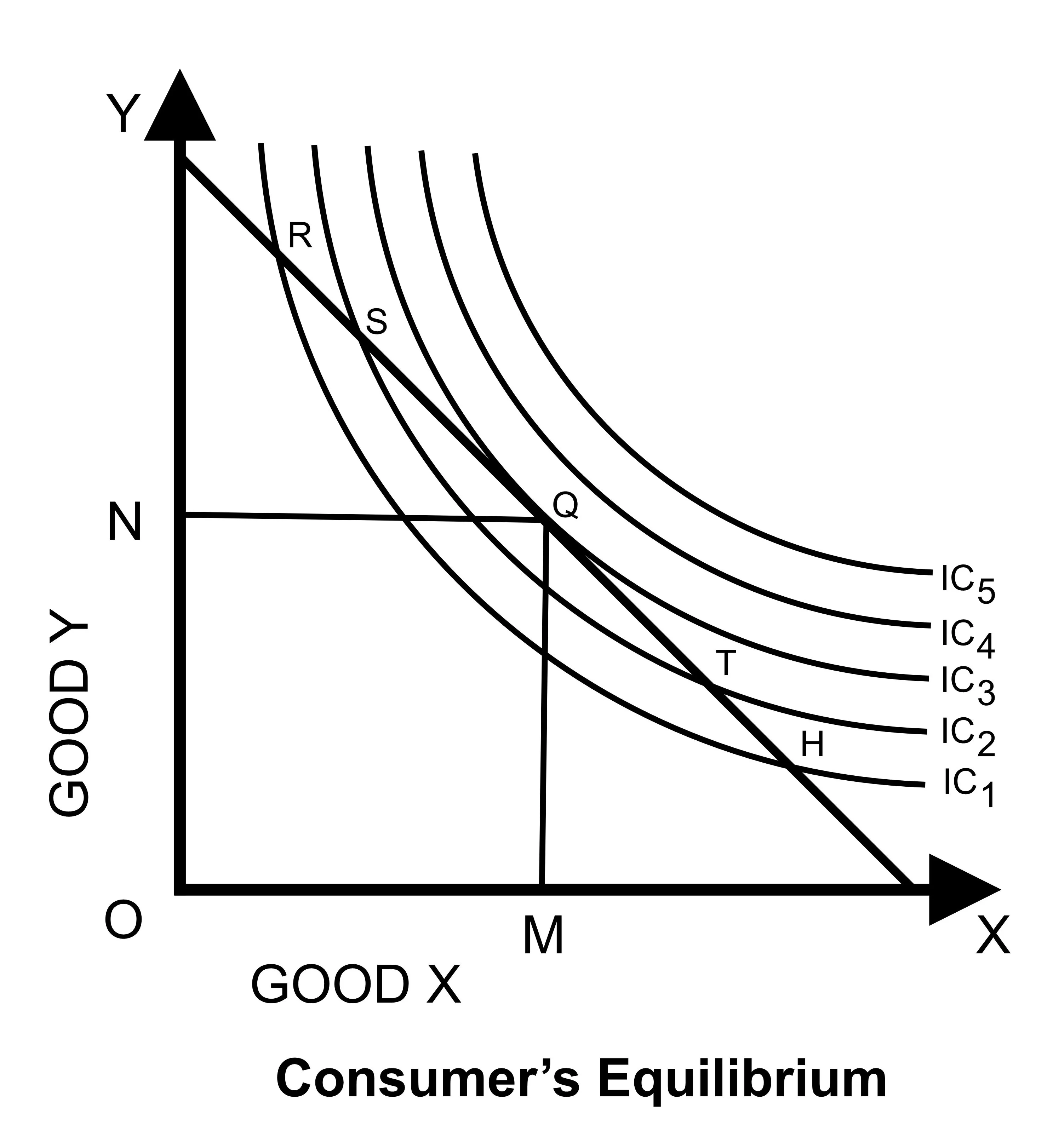
From the figure, we can see that the combinations R, S, Q, T, and H cost the same to the consumer. In order to maximize his level of satisfaction, the consumer will try to reach the highest indifference curve. Since we have assumed a budget constraint, he will be forced to remain on the budget line.

Let’s say that he chooses the combination R. From Fig. 1, we can see that R lies on a lower indifference curve – IC1. He can easily afford the combinations S, Q, or T which lie on the higher ICs. Even if he chooses the combination H, the argument is similar since H lies on the curve IC1 too.

Next, let’s look at the combination S lying on the curve IC2. Here again, he can reach a higher level of satisfaction within his budget by choosing the combination Q lying on IC3 – higher indifference curve level. The argument is similar for the combination T since T lies on the curve IC2 too.

Therefore, we are left with the combination Q.

This is the best choice since Q lies on his budget line and pts puts him on the highest possible indifference curve, IC3. While there are higher curves, IC4 and IC5, they are beyond his budget. Therefore, he reaches the equilibrium at point Q on curve IC3.

Notice that at this point, the budget line PL is tangential to the indifference curve IC3. Also, in this position, the consumer buys OM quantity of X and ON quantity of Y.

Since point Q is the tangent point, the slopes of line PL and curve IC3 are equal at this point. Further, the slope of the indifference curve shows a marginal rate of substitution of X for Y (MRSxy) equal to MUxMUy. Also, the slope of the price line (PL) indicates the ratio between the prices of X and Y and is equal to PxPy

Income-consumption Curve

If the different equilibrium points of consumers resulting from the change in income are added then we will get a curve called Income Consumption Curve (ICC). Thus, ICC is the locus of consumer equilibrium points at various levels of consumer’s income when the price of goods, consumer’s tastes, preferences, habits, etc. remain constant. ICC shows a set of optimal consumption points formed by a change in income keeping price constant.

Income Effect and Derivation Income Consumption Curve in Different Goods

The effect of change in income on the consumer’s consumption decision is different for different goods and services. Here the income effect in the case of different goods is explained in brief.

Income Effect in the Case of Normal Good

In economics, normal goods are any goods for which demand increases if income increases and falls if income decreases holding price constant. It means there is positive income elasticity of demand in the case of normal goods.

In the case of normal goods, there is a positive income effect. It means the quantity demanded increases with the increase in income and vice versa. The income consumption curve (ICC) is upward sloping for normal goods. Let’s consider that both of the goods X and Y are normal goods and see the effect of change in income on the consumption decision with the help of the following diagram.

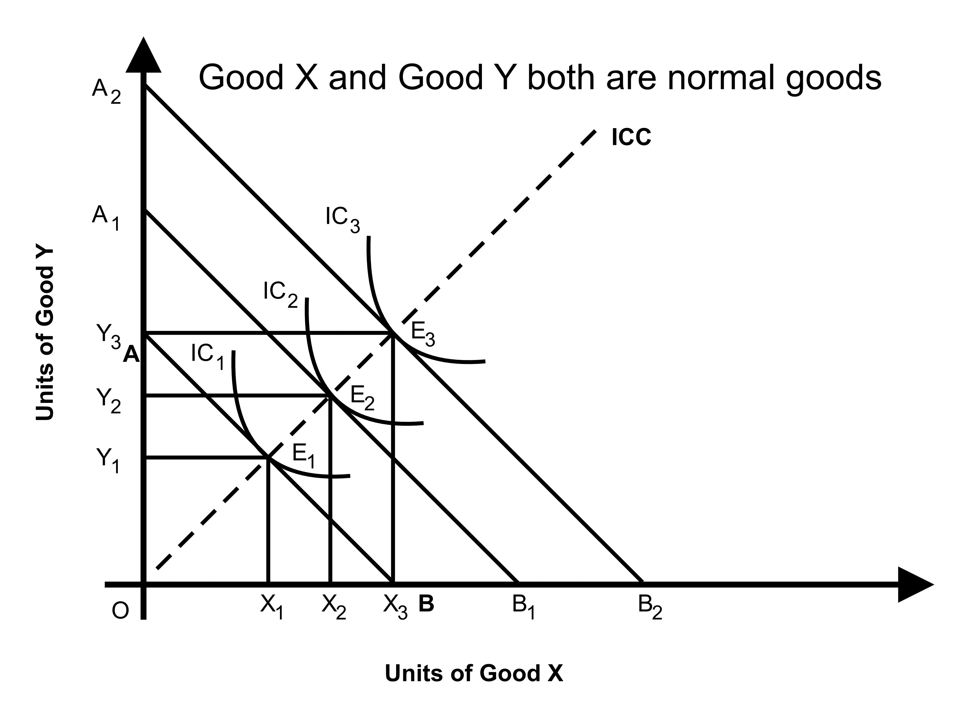
In the above figure, good X is shown along the x-axis and good Y is shown along the Y-axis. AB is the initial budget line and the consumer is in the equilibrium at point E1 on the indifference curve IC1. At the equilibrium point, the consumer has purchased X1 and Y1 units of good X and Y respectively.  

Suppose that there is an increase in income for the consumer. As a result of the increase in income, the budget line of the consumer shifts outward and becomes A1B1. Now, with the A1B1 budget line consumer is in equilibrium at point E2 on a higher indifference curve IC2. At such an equilibrium, the consumer has increased the quantity demand for good X and Y both. Again, if there is an increase in income the consumer’s budget line further shifts towards the right and the consumer attains equilibrium on higher indifference curve IC3. At equilibrium E3, the consumer has further extended his demand for both of the goods.

If we join all the equilibrium points, we get an upward sloping curve and which is known as the income consumption curve (ICC). With the increase in income, the consumer has increased his demand for both goods X and Y and as a result, the ICC is upward sloping. Therefore, if the goods in consideration are normal and there is a change in income the consumption decision will also change positively.

Income Effect in the Case of Inferior Good

In economic theory, an inferior good is a good the demand for which decreases with an increase in consumer’s income assuming price remains constant. A cheaper car (Nano Car) is an example of an inferior good as consumers will generally prefer cheaper cars when they have limited income. If income increases the demand for Nano cars will decrease and the demand for costly/luxurious cars will increase.  The economy class ticket is also considered inferior service (Airlines traditionally have three travel classes, First Class, Business Class, and Economy Class-most expensive, high quality, and basic quality).

In the case of an inferior good, there is a negative effect of income and as a result, the income consumption curve (ICC) will become backward bending or negative in slope. Here we are considering good X as inferior with normal good X and similarly, good X is normal good with inferior good Y. The following figures show the income effect in case of an inferior good.

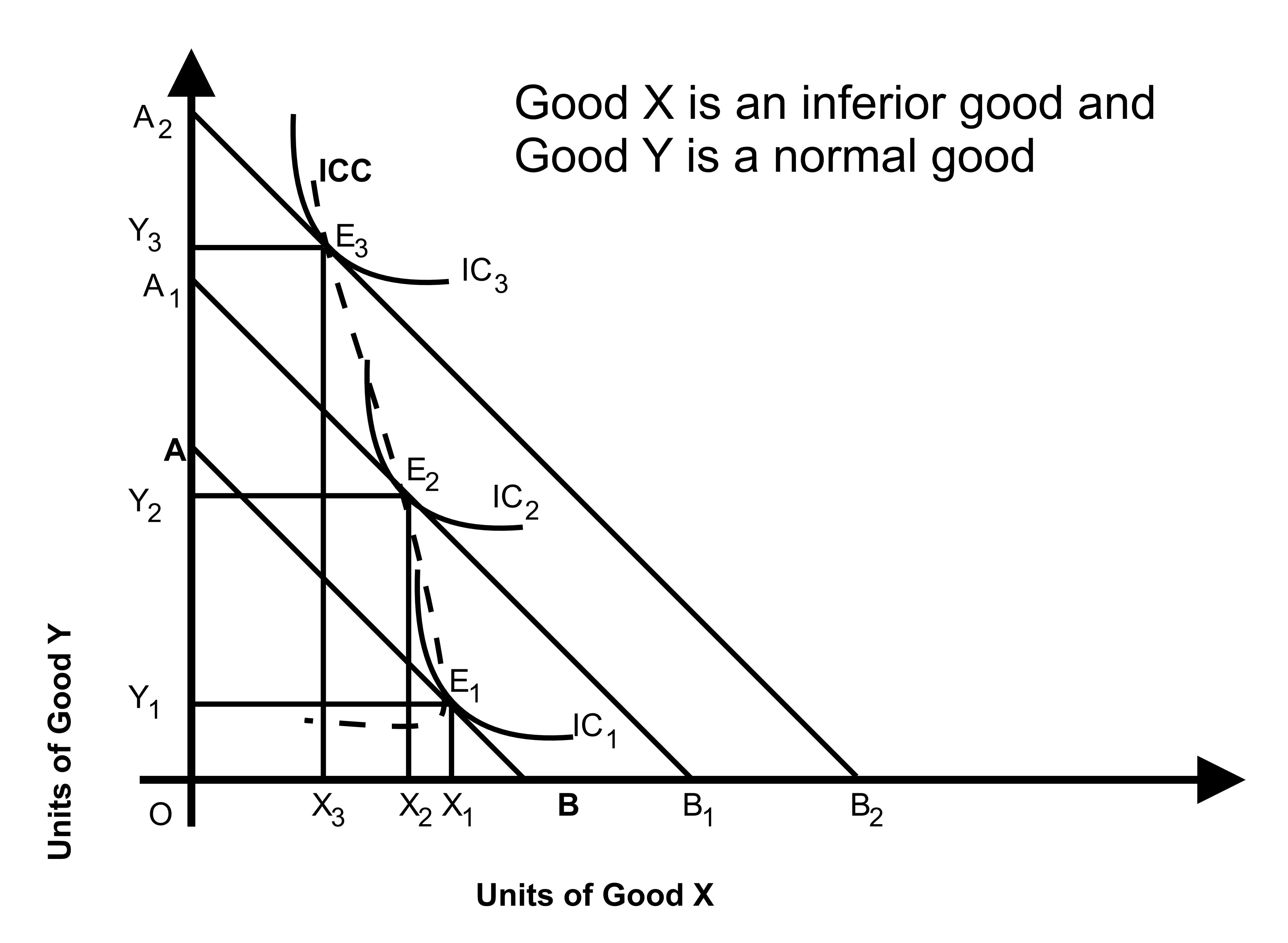
In the first figure, good X is an inferior good and good Y is a normal good. So, with an increase in income, the consumer buys fewer units of good X and more units of good Y. In this case, we obtain backward to the left income consumption curve or negative sloping ICC.  

AB is the initial budget line and the consumer is in the equilibrium at point E1 on the indifference curve IC1. At the equilibrium point, the consumer has purchased X1 and Y1 units of good X and Y respectively.  

When there is an increase in the income then the budget line of the consumer shifts outward and becomes A1B1. Now, with the A1B1 budget line consumer is in equilibrium at point E2 on a higher indifference curve IC2. At such an equilibrium, the consumer has increased the quantity demand for good Y and reduced the demand for good X.

Again, if there is an increase in income the consumer’s budget line further shifts towards the right to A2B2 and the consumer attains equilibrium on higher indifference curve IC3. At equilibrium E3, the consumer has further extended his demand for good Y and reduced the demand for good X.

If we join all the equilibrium points in the first figure, we get a backward bending income consumption curve (ICC). Thus, in the case of inferior good (if inferior good is measured along the X-axis), the ICC will bend backward or towards the Y-axis.

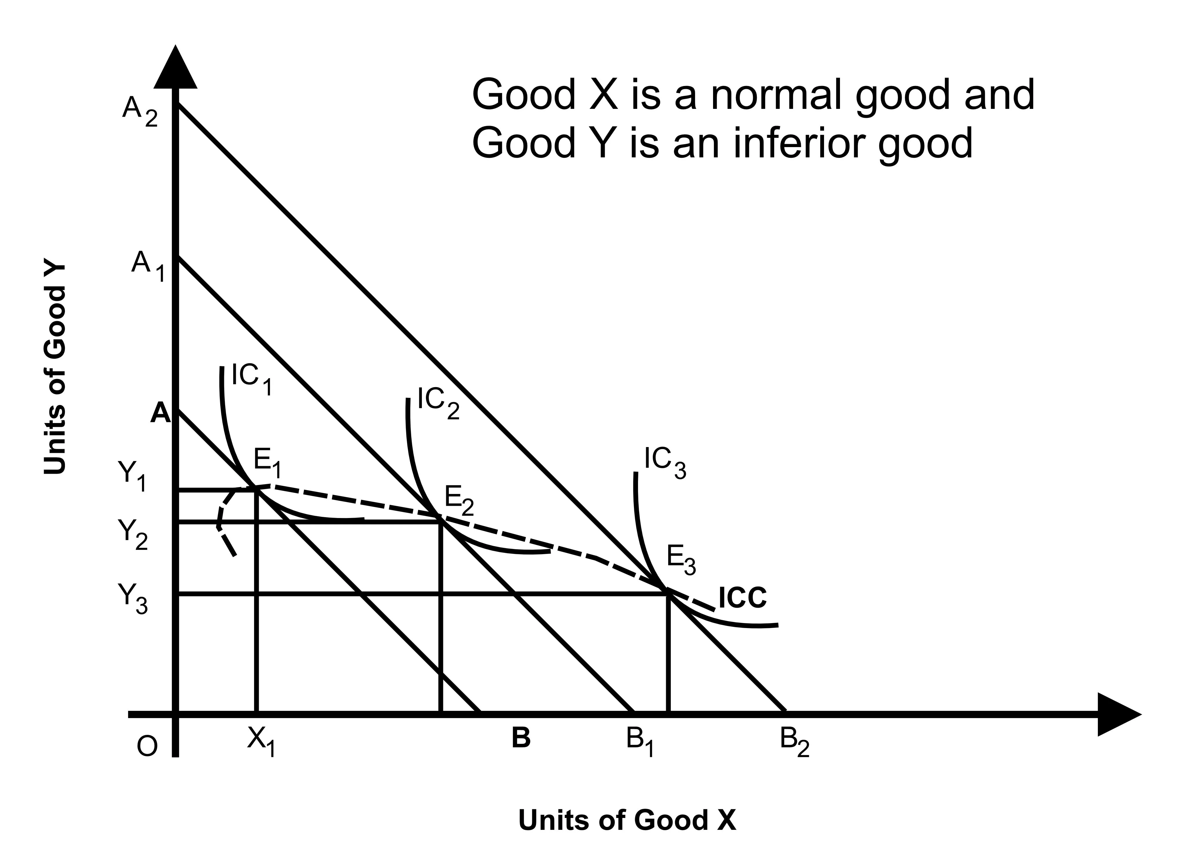
Similarly, in the second figure, we have shown the inferior good on the Y-axis and here we have assumed good Y as an inferior good and good X as a normal good. In this case, there is a continuous increase in the demand for good-X and a fall in demand for good Y with the increase in increase. If we add so obtained equilibrium points then we will get the downward bending income consumption curve (ICC), or ICC bends towards the X-axis.

The Case of Neutral Goods  

In economics, neutral goods are goods that have a demand that is not dependent on the income level. Treatment medicines, salt, cooking oil, etc. are an example of neutral goods. The demand for neutral goods will not change with a rise/fall in income. Thus, the good is neutral good for which the consumer does not care about the consumption at all levels of income. ICC is parallel to Y-axis or a vertical if neutral good is measured along with X-axis and ICC is parallel to X-axis or a horizontal if neutral good is measured along the Y-axis.

The following figures show the income consumption curve (ICC) in the case of neutral goods measured along the X-axis and Y-axis respectively.

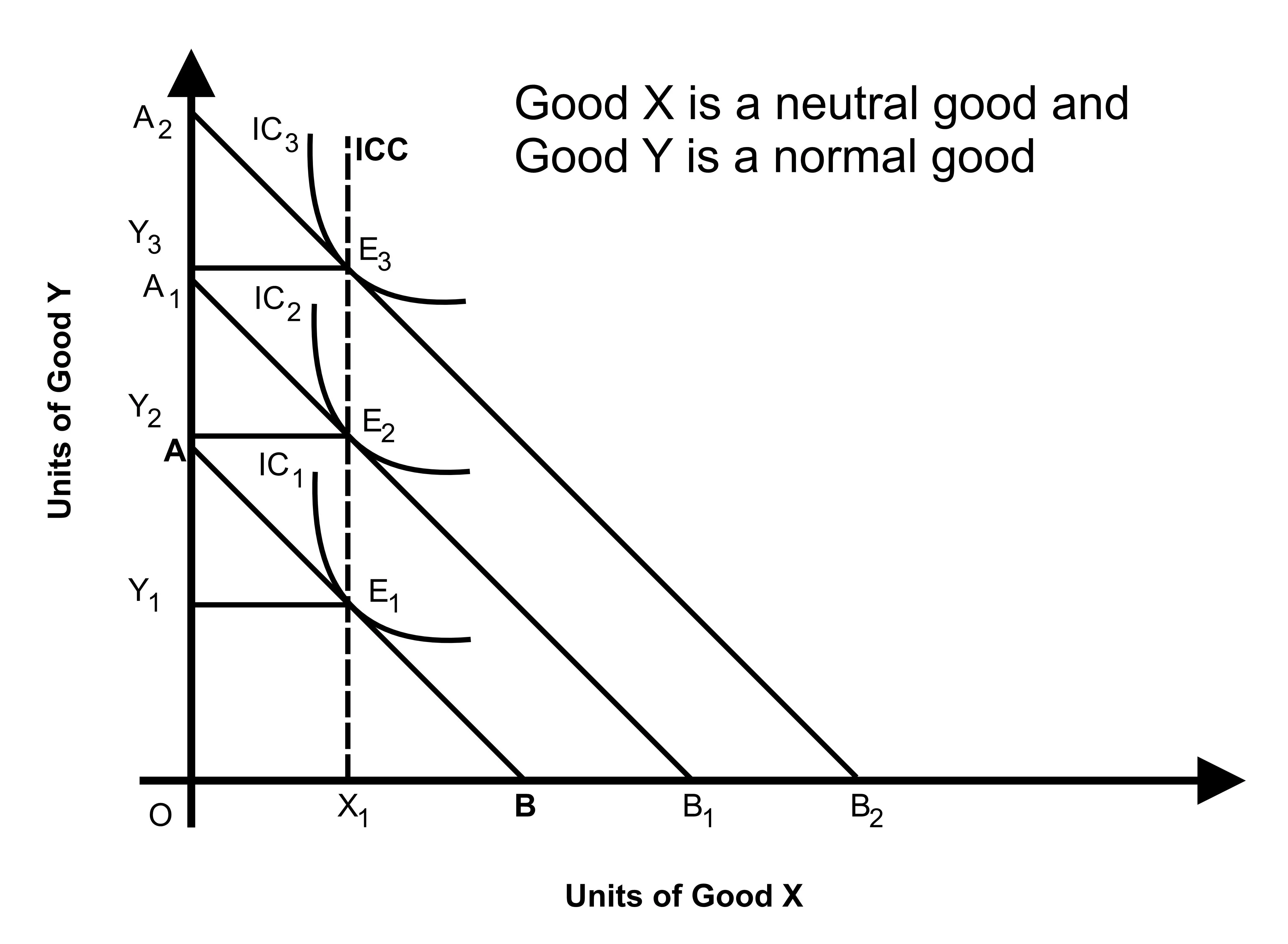
The figure first shows that the neutral good is measured on X-axis or in our case good X is neutral good. AB is the initial budget line and the point E1 is the equilibrium of the consumer on the indifference curve IC1. At the equilibrium point, the consumer has purchased X1 and Y1 units of good X and Y respectively.  

When there is an increase in the income then the budget line of the consumer shifts outward and becomes A1B1. Now, with the A1B1 budget line consumer is in equilibrium at point E2 on a higher indifference curve IC2. At such an equilibrium condition, the consumer has increased the quantity demand for good Y only as good X is neutral and its demand is not affected by any change in income.

Again, if there is an increase in income the consumer’s budget line further shifts towards the right to A2B2 and the consumer attains equilibrium on higher indifference curve IC3. At the equilibrium E3, the consumer has further extended his demand for good Y only and there is no change in the demand for good X.

If we join all the equilibrium points in the first figure, we get a vertical income consumption curve (ICC). Thus, in the case of neutral good (if neutral good is measured along the X-axis), the ICC will parallel to the Y-axis.

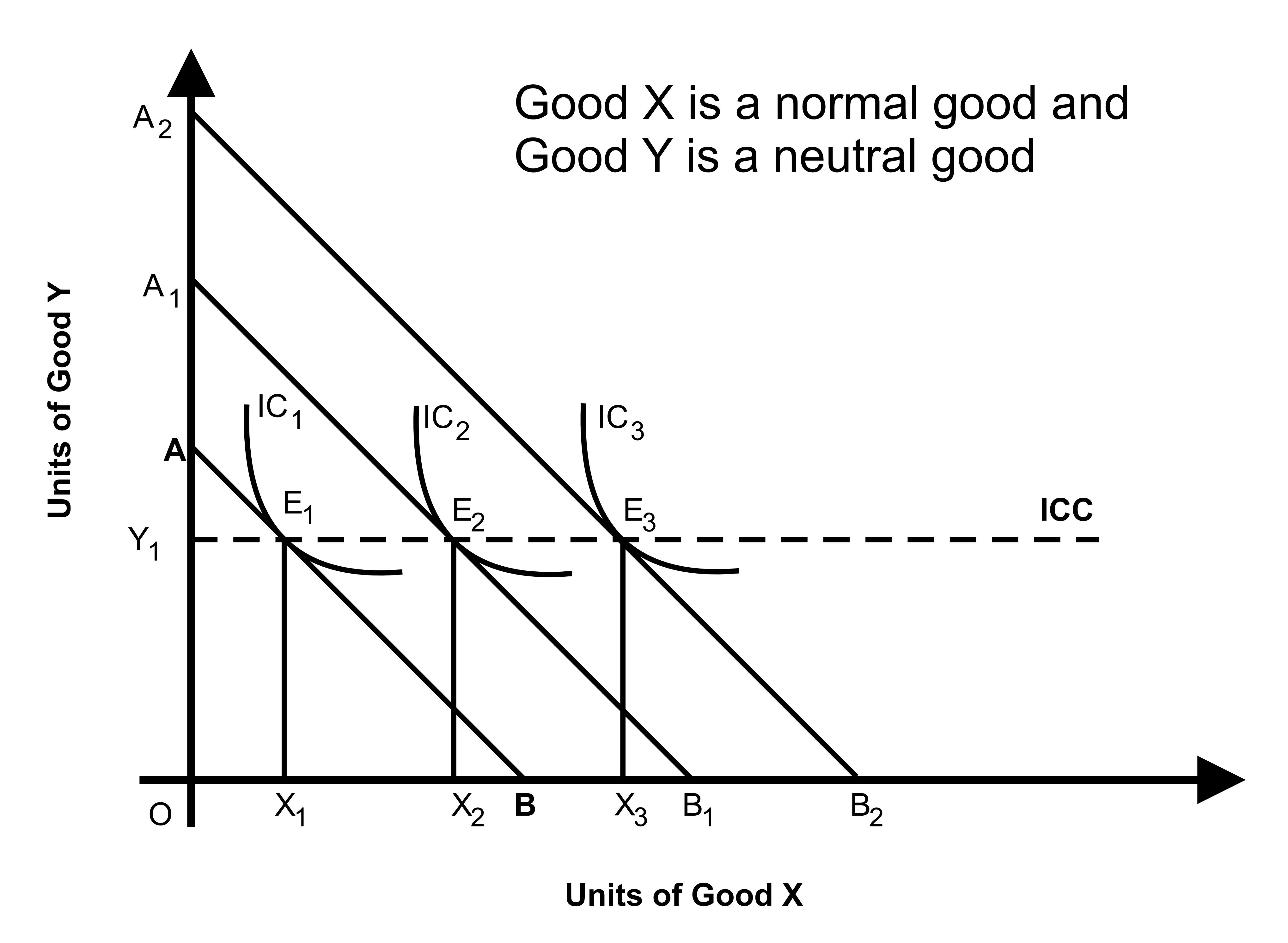
Likewise, in the second figure, we have measured the neutral good along the Y-axis and the normal good along the X-axis. It means in our case good Y is now neutral and good X is a normal good. In this case, there is a continuous increase in the demand for good-X and the demand for good Y remains the same at every level of income. If we add all the equilibrium points then we get the horizontal income consumption curve (ICC), or ICC will parallel to the X-axis.